From Visual Affinity to Learning Credit in Multimodal Reinforcement Learning

Yuhang Han; Dingning Liu; Yujie Chen; Yaojie Zhang; Jingwei Song; Zequn Yang; Xuanming Shang; Li Ding; Zhijiang Guo; Linfeng Zhang

MULTIMODAL REINFORCEMENT LEARNINGarXiv:2610.32324

From Visual Affinity
to Learning Credit.

in Multimodal Reinforcement Learning

Yuhang Han^1,2,3,*Dingning Liu^4,*Yujie Chen^1,2Yaojie Zhang⁴Jingwei Song²

Zequn Yang^2,3Xuanming Shang^2,3Li Ding^2,3Zhijiang Guo^1,†Linfeng Zhang^2,†

¹The Hong Kong University of Science and Technology (Guangzhou)

²Shanghai Jiao Tong University³Shadow Weave

⁴University of Electronic Science and Technology of China

^*Equal contribution.^†Corresponding authors.

A visual connection is a measurement. How it should guide learning depends on the outcome. OVC connects the two with outcome-conditioned, token-level credit.

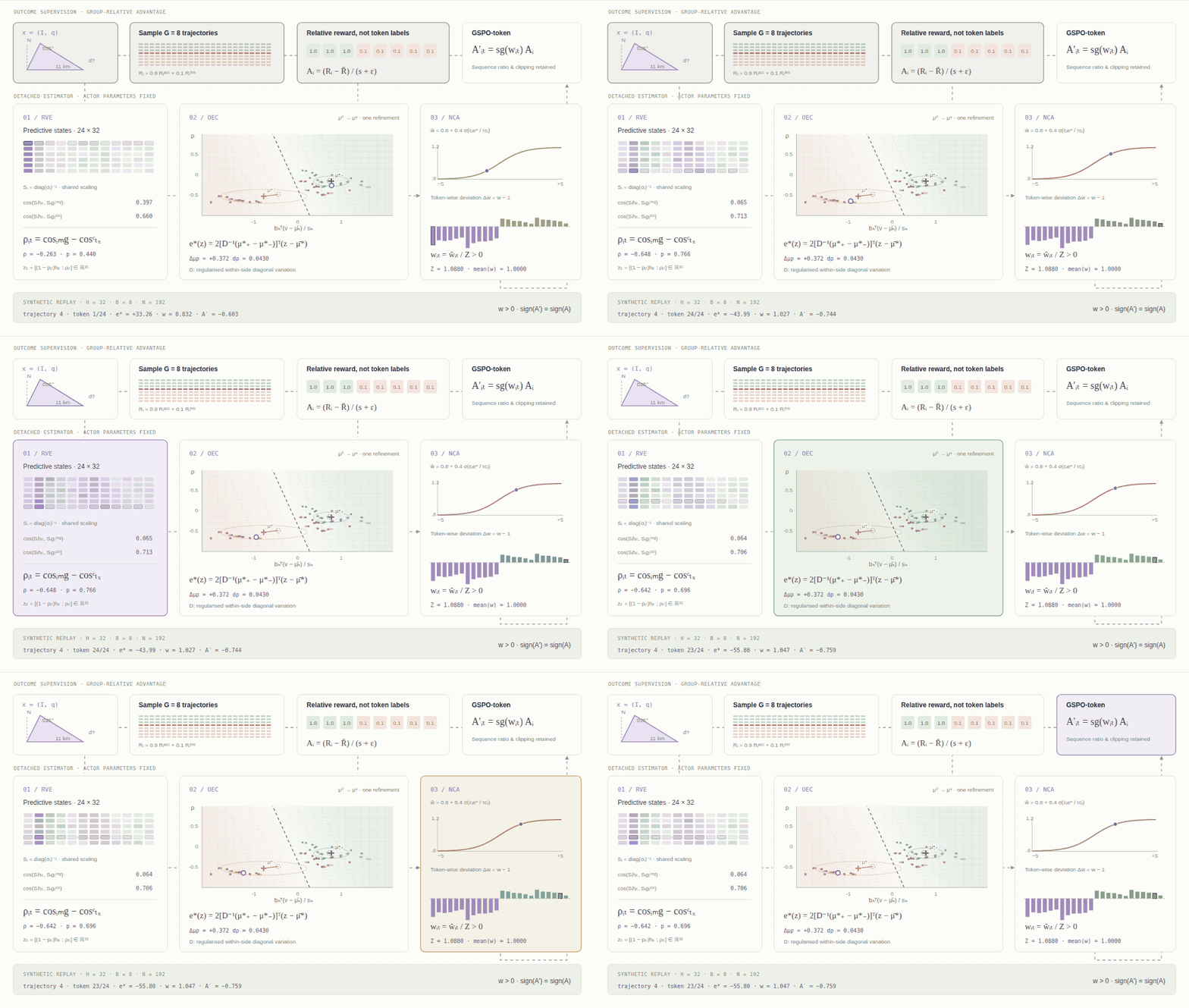
Read the paper Explore the mechanism

THE IDEA, IN MOTIONVisual signalOutcome evidence

Swipe to inspect the full computational graph →

+1.86–2.39pp

Six-task mean gain over GSPO

3 backbones

Qwen3-VL 4B / 8B · Qwen3.5 9B

0 extra modules

At inference time

01 / THE MOTIVATION

One outcome.
Different roles along the way.

A multimodal response mixes observation, interpretation and reasoning. A single response-level advantage cannot say which part should receive a stronger update.

GEOMETRIC REASONING · COORDINATE FRAMES

Q is 11 km due east of P. R is 8 km from P at a clockwise bearing of 025° from north. Find the distance QR.

Verified geometric solutiond = 10.52 km

Aᵢ < 0

A failed final answer does not localise the failure. The bearing observation may be valid even when the frame conversion or a later algebraic operation is wrong.

Constructed surveying example; feature coordinates in the replay are synthetic. Valid/error labels explain the example and are never inputs to the OVC estimator. Advantage signs reflect relative rewards, not token correctness.

Affinity needs a reference.

A predictive state can align with both image representations and the prompt. Absolute image similarity alone does not isolate visual association relative to the surrounding context.

Update direction matters.

The same positive weight strengthens learning in a positive-advantage response and strengthens suppression in a negative-advantage response. An unconditional visual bonus ignores that difference.

Measurement needs calibration.

OVC asks how features differ across advantage sides, relative to within-side variation. Visual association contributes evidence only through those observed outcome contrasts.

EVIDENCE BEHIND THE QUESTION

In the paper’s frozen-model analysis, image-affinity quartiles have accuracies of 80.2%, 77.8%, 82.2% and 79.8%. The highest-affinity group is not the most accurate. Context affinity also distinguishes outcome statistics among pairs approximately matched on image affinity.

Figure 1 · arXiv ↗

02 / THE MECHANISM

Measure. Calibrate.
Then allocate.

OVC is a detached credit estimator built on existing rollouts. It changes the strength of token updates while retaining the original advantage sign and GSPO sequence-level clipping.

01 / RVE

Relative Visual Encoding

Contrast image and non-image prompt affinity using the same response-wise diagonal scaling. The prompt prototype comes from the original multimodal input, not a second text-only forward.

ρ_it = cos(Sᵢh_it, Sᵢg^imgᵢ)
− cos(Sᵢh_it, Sᵢg^ctxᵢ)

No mean subtraction in the cosine. The same scaling is applied to the state and both prototypes.

02 / OEC

Outcome-conditioned Evidence Calibration

Combine the relative visual coordinate with v = (1 − p)h, where p is the sampled token’s probability under the current actor. Compare the joint feature with positive- and negative-advantage reference means under a regularised diagonal within-side metric.

z = [(1 − p)h; ρ]
e(z) = ‖z − μ₋‖²_D⁻¹ − ‖z − μ₊‖²_D⁻¹

Advantage-magnitude-weighted statistics; one soft reference refinement. The metric and pre-refinement margin scales remain fixed.

03 / NCA

Normalized Credit Allocation

Map signed evidence cᵢe(z) to positive raw weights. Normalize across all valid actor-mini-batch tokens, then multiply the response advantage by the detached token weight.

ŵ = λ_min + (λ_max − λ_min) σ(cᵢe/τ_cᵢ)
w = ŵ / mean_tokens(ŵ), A′ = sg(w)A

Global mean weight = 1. This preserves signs, not the norm of the resulting policy gradient. Zero-advantage tokens remain in the normalization.

COMPUTATIONAL WORKBENCH

From representation geometry to update strength.

H = 32 · N = 192

Injected visual–outcome coupling κ+0.60

−1.000+1.00

Within-side shrinkage η0.10

0.000.501.00

Inspect a trajectory

Re-estimated over both sides of the actor mini-batch.

κ perturbs the synthetic visual–outcome association; it is not an OVC training hyperparameter. η controls variance shrinkage. Reference statistics, the metric and normalization are recomputed after each adjustment.

Outcome-discriminative feature geometry

192 TOKENS

The horizontal axis projects all 32 predictive coordinates onto their calibrated direction; the vertical axis is relative visual affinity. The dashed line is zero evidence, not a correctness boundary.

Conditional visual-credit sensitivity

FIXED STATISTICS

Sweep ρ while fixing the predictive feature at its reference midpoint and holding μ*, D, τ and Z fixed. The slopes reverse with the advantage sign; this is a conditional illustration, not causal attribution.

ALLOCATION ALONG THE REASONING TRACE

Compare allocation along the same reasoning trace.

Inspect the estimator: reference moments, metric and one refinement

μ⁰c = Σ_Tc |Aᵢ| zᵢₜ / M_c → q_k = Σ_c Var_|A|,c(z_k)

d_k = max((1 − η)q_k + ηq̄ + ε, r_minq̄ + ε), q̄ = mean(q₁, …, q_H)

u⁰ᵢₜ = σ(cᵢe⁰(zᵢₜ) / τ_cᵢ), μ*c = Σ |Aᵢ| u⁰ᵢₜ zᵢₜ / Σ |Aᵢ| u⁰ᵢₜ

All geometry, features and allocation curves here are computed from a synthetic H=32, B=8, T=24 batch, not extracted from a trained model. The estimator follows Eqs. (1)–(12), including response-wise scaling, advantage-magnitude reference weights, within-side diagonal variation, one refinement and global normalization. The paper’s 9B recipe uses H=4096. Conditional curves keep reference statistics and Z fixed; the batch charts recompute them. The affinity-ranked curve is an illustrative heuristic, not a reproduction of a named baseline. No accuracy trends or empirical results are simulated.

Look inside a training update

Four statistics passes. One policy update.

Aggregate detached advantage-weighted reference moments and construct the regularised diagonal metric.
Estimate the two margin scales using the initial references.
Perform one soft reference refinement, keeping the metric and margin scales fixed.
Compute the global raw-weight mean over all valid tokens.
Recompute differentiable log probabilities; apply detached credit through GSPO-token, accumulate gradients, and update the actor once.

What the method does and does not infer

The actor is fixed between the five passes. Reference groups use the sign of group-relative advantage; the supplied reward mixes accuracy and format. These groups are not token-correctness labels. The estimator is diagonal, not a full-covariance model, and does not establish causal token attribution.

The derivation assumes both advantage sides have positive mass. If all rollout groups have constant rewards, advantages and the policy gradient are zero. The reported formulation concerns image-conditioned inputs.

Algorithm 1 · Appendix F ↗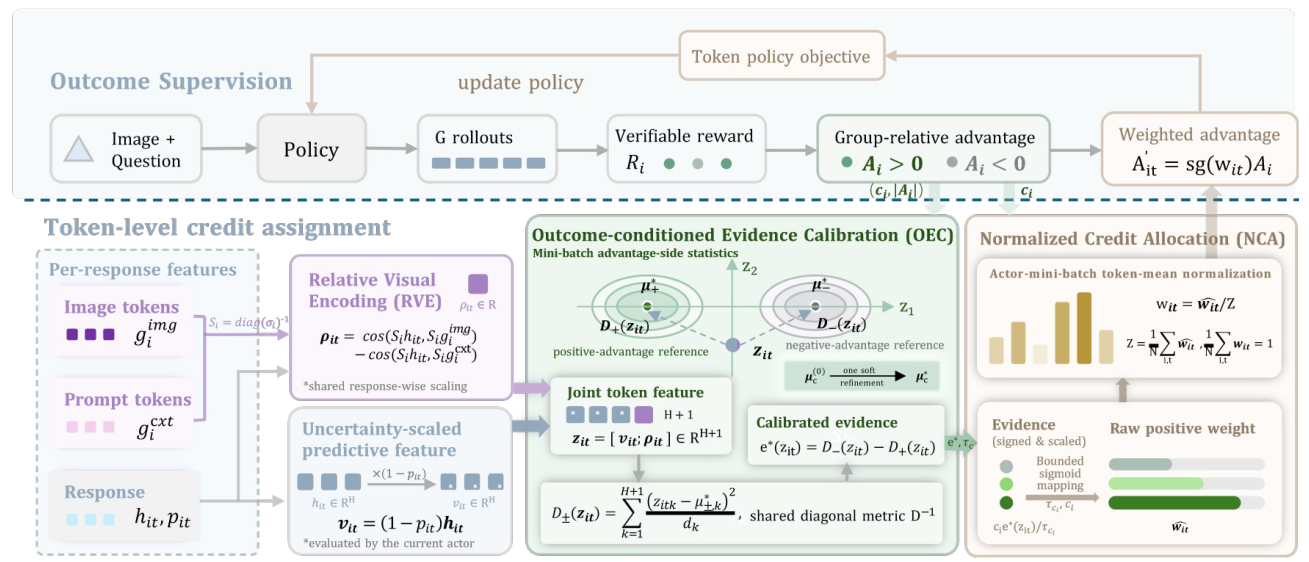

Original OVC framework from Figure 2: outcome supervision above relative visual encoding, outcome-conditioned evidence calibration and normalized credit allocation. — The full framework, reproduced from Figure 2 of the supplied manuscript.↗

03 / THE EVIDENCE

A consistent gain.
Across three backbones.

The same instruction-tuned initialization, RL data and rollout configuration are shared within each model setting. Numbers below are reported in Table 1, averaged over four independent runs.

Qwen3-VL-4B+2.04pp

58.67 → 60.71

Qwen3-VL-8B+2.39pp

61.59 → 63.98

Qwen3.5-9B+1.86pp

68.92 → 70.78

Six-benchmark arithmetic mean: GSPO → GSPO + OVC. Gains are percentage points, not relative percentages. The 9B model uses a different, larger training dataset.

Download data ↓

Benchmark-level change over GSPO

PERCENTAGE POINTS

Main benchmark results from Table 1. All scores are percentages.
Method	MMMU	MathVision	We-Math	MathVista	MMK12-val	MathVerse	Average
Base	48.78	24.67	80.23	74.40	64.46	62.84	59.23
GSPO	44.56	27.30	83.33	76.10	74.73	63.53	61.59
DelTA	49.21	24.01	85.40	77.03	77.06	64.82	62.92
VPPO	49.43	27.69	84.36	76.21	75.29	64.09	62.85
AT-RL	OOM
GSPO + OVC	49.56	29.93	83.45	76.97	78.94	65.05	63.98

READ THE RESULTS WITH THE RIGHT SCOPE

The six-task mean improves for every evaluated backbone, but individual tasks do not all improve: on Qwen3.5-9B, MathVerse drops by 0.94 points versus GSPO. DelTA also remains stronger on 8B We-Math. OVC’s claim is a stronger overall average under the reported settings, not universal benchmark dominance.

OBSERVED TRAINING DYNAMICS

Beyond a final-checkpoint comparison.

In the manuscript’s Qwen3.5-9B run on Math77K, OVC generally achieves higher training reward and MMK12-val performance over the training trajectory. These are the original reported curves, not a reconstructed or simulated time series.

Figure 5 · arXiv ↗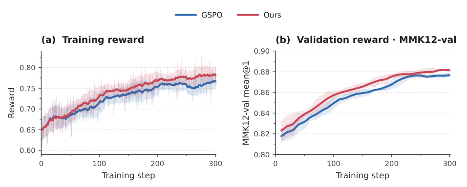

Original Figure 5: GSPO in blue and OVC in red, showing measured training reward and MMK12-val reward over 0–300 training steps. — Original axes and curves retained. Blue: GSPO · Red: OVC. Qwen3.5-9B / Math77K.

BEYOND NONUNIFORM WEIGHTS

The token–weight correspondence matters.

Averaging weights within each response loses 1.48 points. Permuting them loses 1.56 points, even though each response keeps exactly the same weight multiset. The gain depends on where the weights go.

Table 2 · Qwen3-VL-8B · Four-task mean, not the six-task average above. Full OVC: 63.85; GSPO: 62.57.

Why the visual coordinate and calibration need to work together

With within-side calibration, adding the visual coordinate raises the mean from 61.98 to 63.85. With an identity metric, it lowers the mean from 62.29 to 62.10. This interaction cautions against treating visual affinity as an independently beneficial bonus.

AblationChange from full OVC

No visual coordinate

−1.87

Absolute image affinity

−1.62

Identity metric

−1.75

Response-mean weights

−1.48

Within-response permutation

−1.56

Affinity-ranked weights

−1.58

04 / TRAINING-TIME ONLY

Reuse the rollout.
Keep inference unchanged.

OVC adds no learnable head, auxiliary reward model or process annotations. Its additional computation is in detached training statistics, not in the inference graph.

5.16%

of the measured training step spent on OVC-specific passes

OVC statistics189 s / 3,663 s

Figure 4 reports a single complete training step. This is a share of total step time, not a universal slowdown or an inference-time overhead.

05 / GO DEEPER

Read the full story.

Derivations, evaluation protocols, complete ablations and the actor-update algorithm are in the manuscript and its supplement.

Full paper & supplement

Method & derivations§3 / App. B–E ↗Results & ablationsTables 1–2 ↗Actor-update algorithmAlgorithm 1 ↗Mechanism animationGIF ↓

BIBTEX CITATION

@misc{han2026visualaffinitylearningcredit,
  title={From Visual Affinity to Learning Credit in Multimodal Reinforcement Learning},
  author={Yuhang Han and Dingning Liu and Yujie Chen and Yaojie Zhang and Jingwei Song and Zequn Yang and Xuanming Shang and Li Ding and Zhijiang Guo and Linfeng Zhang},
  year={2026},
  eprint={2610.32324},
  archivePrefix={arXiv},
  primaryClass={cs.AI},
  url={https://arxiv.org/abs/2610.32324},
}

Use the BibTeX above to cite arXiv:2610.32324. Paper links open the arXiv record.

From Visual Affinityto Learning Credit.

One outcome.Different roles along the way.